Investors hate to realize capital gains. After realizing capital gains and paying the tax, investors have less proceeds available to reinvest lessening their potential for future compounded growth. All things being equal it is better not to realize the capital gains and delay sales as long as possible. The investor may die and get a step up in cost basis. Or the investor may decide to sell the stock a decade later and receive a decade’s worth of growth on the money they would have otherwise had to use to pay the tax.

But what if the investment they are holding is inferior to another investment they would prefer to be invested in? Perhaps the new investment is superior because it has a lower expense ratio, or perhaps it is in an asset class or sector which has a greater expected investment return. How much better does the new investment’s prospects have to be to overcome having to sell an otherwise highly appreciated investment?

The capital gains tax is an economic roadblock. It traps capital in inefficient locations as investors don’t want to lose 15% of their wealth simply because they want to rebalance or change their investment strategy. However, sometimes it pays to jump over the roadblock. Sometimes, losing the 15% while leaping the hurdle pays off.

These calculations are called “Hurdle Table Calculations,” and the mathematics may surprise you.

Take a concrete example:

A Concrete Example

You hold $10,000 of stock investment ABC with an appreciation of 50% which you expect to have a 8% nominal return in a 2.1% inflationary environment. The inflationary environment does not matter for these calculations, I am including it simply to justify an 8% nominal return. On the one hand the investor does not want to sell the highly appreciated stock position because they are subject to the 15% federal capital gains rate and the 5.75% Virginia state capital gains rate for a total capital gains tax burden of 20.75%. On the other hand the investor has an investment option XYZ that they would like to move into in which they believe they will earn more than 8%.

The cost basis for the $10,000 in ABC is $6,666.67, making the capital appreciation $3,333.33 (50%).

If they sell the ABC investment now, they will owe $691.67 in capital gains taxes (20.75% of $3,333.33) and only have $9,308.33 of proceeds available to reinvest.

If they let the $10,000 continue to grow in ABC, after 10 years at 8% it will be worth $21,589.25.

After those 10 years pass, they might sell the stock. If they do, the investor will have a capital gain of $14,922.58 ($21,589.25 minus $6,666.67) and at a 20.75% capital gains tax, they will owe $3,096.44. Meaning, after taxes they will be left with $18,492.81.

If they sold ABC now, purchased the new XYZ investment, and XYZ could appreciate to $20,897.58, the investor would have a capital gain of $11,589.25 ($20,897.58 minus $9,308.33) on XYZ. They would owe $2,404.77 in capital gains tax (20.75% of $11,589.25). After paying the capital gains tax the investor would be left with $18,492.81 ($20,897.58 minus $2,404.77) which is the same as if they continued to hold ABC for ten years.

In order for $9,308.33 to grow to $20,897.58 after ten years, the rate of return of XYZ would have to be 8.42% or 0.42% higher than ABC.

If however, the ABC owner dies after 10 years, then they would have gotten a step up in basis and owe no capital gains tax on ABC. In that scenario, in order for $9,308.33 to grow to the full value of $21,589.25 after ten years, the rate of return of XYZ would have to be 8.78% or 0.78% higher than ABC.

As you can see from this example, there is a strong case to sell and reinvest a highly appreciated investment if you believe that your new investment is expected to have a modestly higher return. In our example, assuming a sale of assets in ten years or longer the hurdle rate necessary for the new superior investment was just 0.42% better than the old investment. There are many solid reasons to expect a higher return.

A move from large cap to small cap value might expect an investment return as much as 3.48% higher.

A move from a foreign index fund to a strategy which invests in the countries high in economic freedom might expect an investment return as much as 1.28% or more higher.

Simply rebalancing your portfolio might receive a rebalancing bonus as much as 1.6% higher return.

A move to dynamically tilt toward an investment with low forward P/E ratios might expect to receive an investment return as much as 1.19% higher.

A move out of a higher cost fund into a similar but significantly lower cost investment can expect a return equal to the difference in expense ratios.

For all of these reasons investors should not be shy to realize the capital gains when justified by the math and the expectation. The math to compute the hurdle tables is fairly complex and the remainder of this article will explain how the hurdles are calculated.

The Mathematics of Hurdle Calculations

In the above example, I made calculating the hurdle look easy. I simply stated at the end what the rate of return of XYZ would have to be. However, there is a complex formula to calculating the hurdle rate. To do so, you have to solve for what excess return will produce the same after-tax value when compounded for a specific number of years.

To create a generic hurdle table that can be used on the simplest inputs, imagine that the current value of our formula’s investment is $1 or 100%. Then, the complex hurdle table calculation starts with two simple well known financial formulas.

First, the future value of an investment is the current value times one plus the annual rate of return (r) raised to the number of years (y) or written in math:

(1 + r) ^ y

Second, we need to turn the percent appreciation of an investment into a formula for cost basis. Cost basis is the current value times one divided by one plus the percent appreciation (a) or written in math:

1 / (1 + a)

Using these two formulas, we can create a tax owed formula. Tax Owed is the gain times the tax rate (t). The future value minus the cost basis equals the gain, so using the above formulas this makes the tax owed:

[ ((1 + r) ^ y) – (1 / (1 + a)) ] * t

Then, the future after-tax value of the original asset would be the future value minus the tax owed or:

((1 + r) ^ y) – [ ((1 + r) ^ y) – (1 / (1 + a)) ] * t

Through basic algebra we can simplify the future after-tax value of the original asset to:

[(1 – t) * ((1 + r) ^ y)] + (t / 1+a)

In this way, we now have a generic formula to calculate the future after-tax value of an asset based on its current appreciation, future expected return, number of years, and the investor’s capital gains tax rate. This will be used to calculate the future after-tax value of the asset you are thinking about selling, but we also need to be able to calculate the future value of the asset we could buy with the proceeds of this asset if we sold it.

To do that, we start with the capital gain, which is the value of the investment minus the cost basis. As we are creating generic formulas, the initial investment is 1. That makes the formula:

1 – (1 / (1 + a))

Using basic algebra, this simplifies the capital gain formula to:

a / (1+a)

The initial tax owed is then the capital gains (the above formula) times the tax rate (t) and the proceed available for reinvestment the current value (which is 1) minus the tax owed. Put all together into a formula that makes the proceeds available for reinvestment (which will also be the cost basis of the new investment):

1 – ([a / (1+a)] * t)

This cost basis of the reinvestment can also be written as:

1 – (at / (1+a))

This proceed available for reinvestment is then the new investment’s current value. The future value of an investment is the current value times one plus the annual rate of return (r+e) raised to the number of years (y). This investment’s rate of return might be bigger or smaller than the original rate of return. Thus, the rate of return of this investment is the first fund’s rate of return (r) plus some extra amount (e). That makes the future value of the reinvestment:

(1 – (at / (1+a))) * ((1 + r + e) ^ y)

The taxes owed on selling this future value of the reinvestment would be the above future value minus the cost basis (which was the proceeds available) times the tax rate. In math that means the tax owed on the future value of the reinvestment is:

{ [ (1 – (at / (1+a))) * ((1 + r + e) ^ y) ]  – [ 1 – (at / (1+a)) ] } * t

Through algebra, this simplifies the tax owed on the future value of the reinvestment to:

( t – (a * t^2) / (1+a) ) * ( [ (1 + r + e) ^ y ] – 1)

The after-tax value of the future value of the reinvestment would then be the future value of the reinvestment minus the tax owed. In math this would be:

(1 – (at / (1+a))) * ((1 + r + e) ^ y)
–
( t – (a * t^2) / (1+a) ) * ( [ (1 + r + e) ^ y ] – 1)

Finding The Hurdle Rate

Now that we have these equations, we can solve for what excess return (e) would justify selling the initial investment and reinvesting the proceeds.

Stated another way, the question is: what value of e causes the future after-tax values to be the same after y years?

Now, because it is possible to get a step up in cost basis from death and thus the after-tax value will equal the full future value, we will have two different formulas to solve.

1. Assuming that the investor dies after y years and we receive a step up in cost basis
2. Assuming the investor does not die but instead decides to sell the investment after y years

Those two formulas work out to:

First, the excess return needed if the investor will get a step up in cost basis after y years in its most complex form:

e = ((((1 + r) ^ y) / (1 – ( (1 – (1 / (1 + a))) * t))) ^ (1/y)) – 1 – r

Simplified and legible, the return needed to beat a step up on cost basis is:

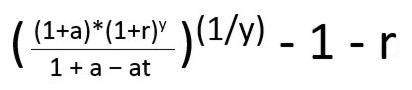
Second, the excess return needed if the investor sells the investment after y years in its most complex form:

e =  (((((1 + r) ^ y) – (( ((1 + r) ^ y) – (1 / (1 + a))) * t) – ((1 – ( (1 – (1 / (1 + a))) * t)) * t)) / ((1 – ( (1 – (1 / (1 + a))) * t)) * (1 – t))) ^ (1 / y)) – 1 – r

Simplified and legible, the return needed to beat realizing the gains after y years is:

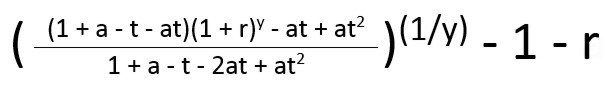
These are complex formulas, but they are valuable calculations that show that there is an expected increase of return which will justify selling even a highly appreciated asset.

Photo by Tim Wright on Unsplash