With all the talk about how, “The market has to correct sometime soon.” and “The market can’t just go up forever, can it?” it is easy to become worried and think you are a fool for remaining invested. You are not.

We recently experienced a drop in the S&P 500 Price Index from September 20, 2018 to December 24, 2018 of -19.78%, just shy of the definition of a Bear Market. So the market had a nice correction and has appreciated since then. Year to date the MSCI USA Large Cap Index (USD) is up 16.07% through September 3, 2019. Normal market movements are inherently volatile.

A year ago, we wrote “S&P 500 Fairly Valued At End Of June 2018” showing that forward P/E ratios suggested that the markets were valued exactly at their historical averages. Many investors were worried then, but over the next year the S&P 500 appreciated 10.42%.

J.P. Morgan offers a quarterly Guide to the Markets which always contains an updated S&P 500 Index Forward P/E Ratio. As of June 30, 2019, the S&P 500 Forward P/E Ratio is 16.74, well within the normal range. The current 25 year average forward P/E ratio is 16.19. One standard deviation ranges from 12.99 to 19.39.

Price per earnings (P/E) comes in many different measurements each based on a different measurement of earnings (E). There is the trailing twelve months of earnings (ttm P/E), the cyclically-adjusted price-to-earnings (CAPE), and the future expected twelve month earnings (forward P/E). Forward P/E is based on an industry consensus of expected earnings. Each measurement has its difficulties, but either CAPE or forward P/E is better than ttm P/E at predicting future appreciation.

Historically when the markets have a low forward P/E, they have a slightly higher expected appreciation. Similarly, when the price of the markets is expensive compared to future expected earnings, they have a slightly lower expected appreciation. In simple terms, when you buy a stock, you are buying an expected stream of revenue. It is better when you can buy that expected revenue stream for less cost.

Although a low forward P/E suggests higher expected appreciation, using this metric does not justify jumping in and out of the markets. Even when the markets are pricey it is still better, on average, to be invested than not to be invested.

While we do not use this metric for market timing, we do use this metric to adjust the target sector allocation of about two dozen strategic underlying categories. We overweight those categories where earnings appear historically cheap and underweight those categories where earnings appear historically expensive.

We do not use J.P. Morgan’s quarterly Guide to the Market for our data. That data is updated quarterly and we update ours monthly. Additionally, we use a longer time period than just the last 25 years for our averages and standard deviations. And finally, we require a data source that includes every category to which we allocate a portfolio. This means we track the forward P/E ratios for everything from stocks in the Netherlands to U.S. healthcare stocks. These details change the numbers, but they do not change the general principle.

It took us awhile to find reliable forward P/E ratio data for all of the different categories. Ultimately, we found the MSCI Fact Sheets which contain data on a host of different MSCI Indexes from the MSCI Singapore Index (USD) to the MSCI New Zealand Index (USD). Currently the Singapore forward P/E ratio is a low 11.95, while the New Zealand forward P/E ratio is a relatively high 26.50. As a result, we are under-weighting New Zealand and over-weighting Singapore in our target allocations.

While it was difficult to find current forward P/E ratio measurements, it was even more difficult for us to find historical forward P/E data sufficient to choose estimates for the long-term average and standard deviation for over two dozen separate equity investment categories. Having found such data, we now adjust asset allocations each month based on the latest data.

For example, instead of the S&P 500 Index, we use the MSCI USA Large Cap Index (USD). As of August 30, 2019, The MSCI Index has a forward P/E ratio of 16.99. We compare this against our average 16.90 and a one standard deviation range from 10.45 to 23.35. Our historical data set must contain some periods which were more volatile than the last 25 years. Using our numbers, if the forward P/E ratio were at 23.35 or higher we would invest just 50% of what we normally would. And if the forward P/E ratio were 10.45 or lower we would invest 150% of what we normally would. There is nothing magical about these percentages. We are trying to gain from dynamically tilting based on the forward P/E ratio without making more than half a mistake.

With a forward P/E ratio between these extremes, we tilt a smaller, proportional amount. With a forward P/E ratio of 16.99, slightly higher than the historical average, we target a slightly lower allocation of 99.30% of what we would normally invest. The math used to compute this value is: 100% + ((16.90 – 16.99) / (23.35 – 10.45)).

J.P. Morgan’s Guide to the Markets has another slide (currently slide 6 of 71) which shows the relationship between the current forward P/E ratio of the S&P 500 and the subsequent 1- and 5-year equity returns. As they explain, “Returns are 12-month and 60-month annualized total returns, measured monthly, beginning June 30, 1994. R² represents the percentage of total variation in total returns that can be explained by forward P/E ratios.”

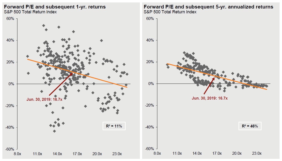
Note that there appears to be a benefit of over-weighting a category when the forward P/E ratio is low and under-weighting it when the forward P/E ratio is high. But although there is a trend line, the scatter plot of actual 12-month data shows that random market noise and other factors often swamp any effect from this valuation metric. In fact, only about 11% of the market’s subsequent 12-month return could be attributable to the forward P/E ratio. Looking at the 5-year subsequent return, however, seems to imply that 46% of the 5-year appreciation is attributable to this valuation metric.

We can also see that until the forward P/E ratio of the S&P 500 Index approaches 22, it is better to be invested than not to be invested. The forward P/E ratio of the S&P 500 Index has not been near 22 since the end of the 1990s.

We haven’t written much about the technical aspects of the dynamic tilt we use in all of our portfolio management since our 2012 article, “Using Dynamic Asset Allocation to Boost Returns.” In that article the annual benefit for a dynamic tilt between the S&P 500 and the Russell 2000 Value was 1.19% annually without changing the average asset allocation and without increasing the standard deviation of the portfolio.

Implementing a dynamic tilt is both complex and simple.

It requires a great deal of thought and data collection to design. But it is as simple as collecting the latest forward P/E ratio information, plugging it into the formulas, and then adjusting our static asset allocation by the dynamic factor we have calculated. After adjustments, the resulting asset allocation may add up to more or less than 100%. We then normalize the percentages within each of the six asset categories back to 100%.

It is another small way to systematize being a contrarian.

Photo by Julian Howard on Unsplash