The Sharpe Ratio is the expected excess return of an investment divided by the standard deviation of that investment.

The “excess return” is the expected return of an investment minus the expected return of a so-called risk-free, guaranteed investment return.

For example, if you expect an investment or a portfolio to have a mean return of 9% and a standard deviation of 12% in an environment where a so-called risk-free, guaranteed investment has a return of 3%, that investment or portfolio’s Sharpe Ratio would be 0.5. The calculation is simply (9% – 3%) / 12%.

The Sharpe ratio is a quick measure that tries to answer the question, “Am I getting enough extra return for my extra risk?”

Unfortunately it is too simplistic a measure to answer that question accurately.

In January of 2016, we wrote an article entitled, “Why Invest In Chile?” We wrote the article because Chile had just experienced three consecutive years of significant negative returns: -23.86% in 2013, -12.73% in 2014, and -18.05% in 2015. It’s cumulative return for 3 years stood at -45.54% and one or two clients were wondering why they and we were still invested in Chile when it was “doing nothing but going down.”

Many investors mistakenly believe that when something has “gone down” (past tense) it is “going down” (present tense). This causes investors to chase returns and under perform the very investments they are invested in, getting in after an investment has already risen and getting out after an investment has already gone down.

We make a distinction between an unfortunate investment and a mistake. An unfortunate investment is one that you have very good reasons to select, but which happens to go down in the short term. A mistake is an investment which you should have known ahead of time was not the right investment choice.

At the end of 2015, Chile was an unfortunate investment, but it was not a mistake. Using historical returns as of the end of 2015 and including the final three negative returns, we showed how the efficient frontier would still suggest having a small allocation to Chile. In fact, if your portfolio was constrained to only include two investments (the S&P 500 and Chile), the efficient frontier would suggest that any allocation less than 12% to Chile was not on the efficient frontier. And that any allocation between 12% Chile and 19% Chile would actually reduce the over all portfolio volatility.

Here is a larger graph of the efficient frontier calculation:

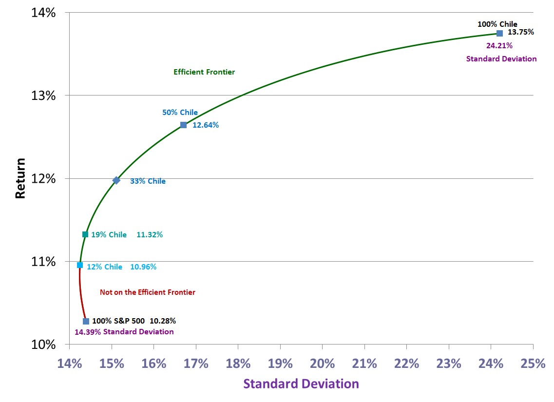
Chile could have had a fourth negative year in 2016, but it did not. In retrospect, our analysis was vindicated. In 2016, Chile had a return of 17.79%. And in 2017, Chile is up an additional 30.19% year to date through August 31, 2017.

By itself Chile is volatile. But in a well-crafted portfolio it can both reduce volatility and increase returns.

This is easier to see when computing an efficient frontier such as the two dimensional graph above. It is much more difficult when trying to use a one dimensional measure such as the Sharpe Ratio.

Using the data used in the graph above and assuming a 3.0% risk-free, guaranteed return, the Sharpe Ratio for the 100% S&P 500 portfolio is 0.5055. The Sharpe Ratio for the 100% Chile portfolio is 0.4440.

By themselves, these two points would suggest that the additional average return of Chile is not worth the additional risk taken.

But if we compute the Sharpe Ratio for each of the blended portfolios starting at 0% Chile (100% S&P 500) and going all the way through 100% Chile (0% S&P 500), the graph of these Sharpe Ratios looks like this:

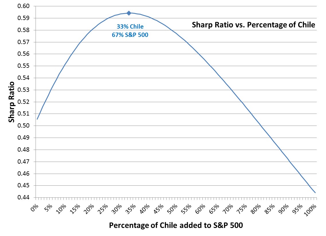
In our first graph, any portfolio between 12% Chile and 100% Chile was on the efficient frontier.

The Sharpe Ratio, however, implies that 33% Chile and 67% S&P 500 is the optimum portfolio and every other choice on the efficient frontier is sub-optimal. That is simply not the case.

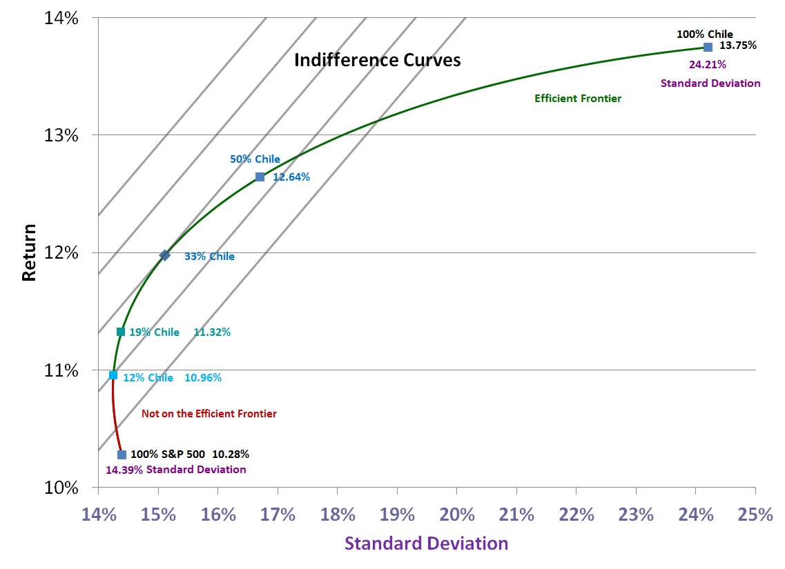
Normally in modern portfolio theory, the optimum portfolio would be the portfolio that is tangential to the investor’s highest indifference curve. Indifference curves are based on an investor’s desire for return and the risk they are willing to take. It is a line which represents risk-return points for which the investor is indifferent, equally wiling to be anywhere along the line. The Sharpe Ratio is simply one of many indifference curves, and it is not a curve, it is a straight line. Here is a visual representation of how the Sharpe Ratio decides that 33% Chile is the optimum portfolio:

If an investor was more willing to tolerate short term risk (annual standard deviation) in order to seek return, their indifference curve might suggest a higher allocation to Chile. Here is a set of straight line indifference curves which would suggest a 50% allocation to Chile:

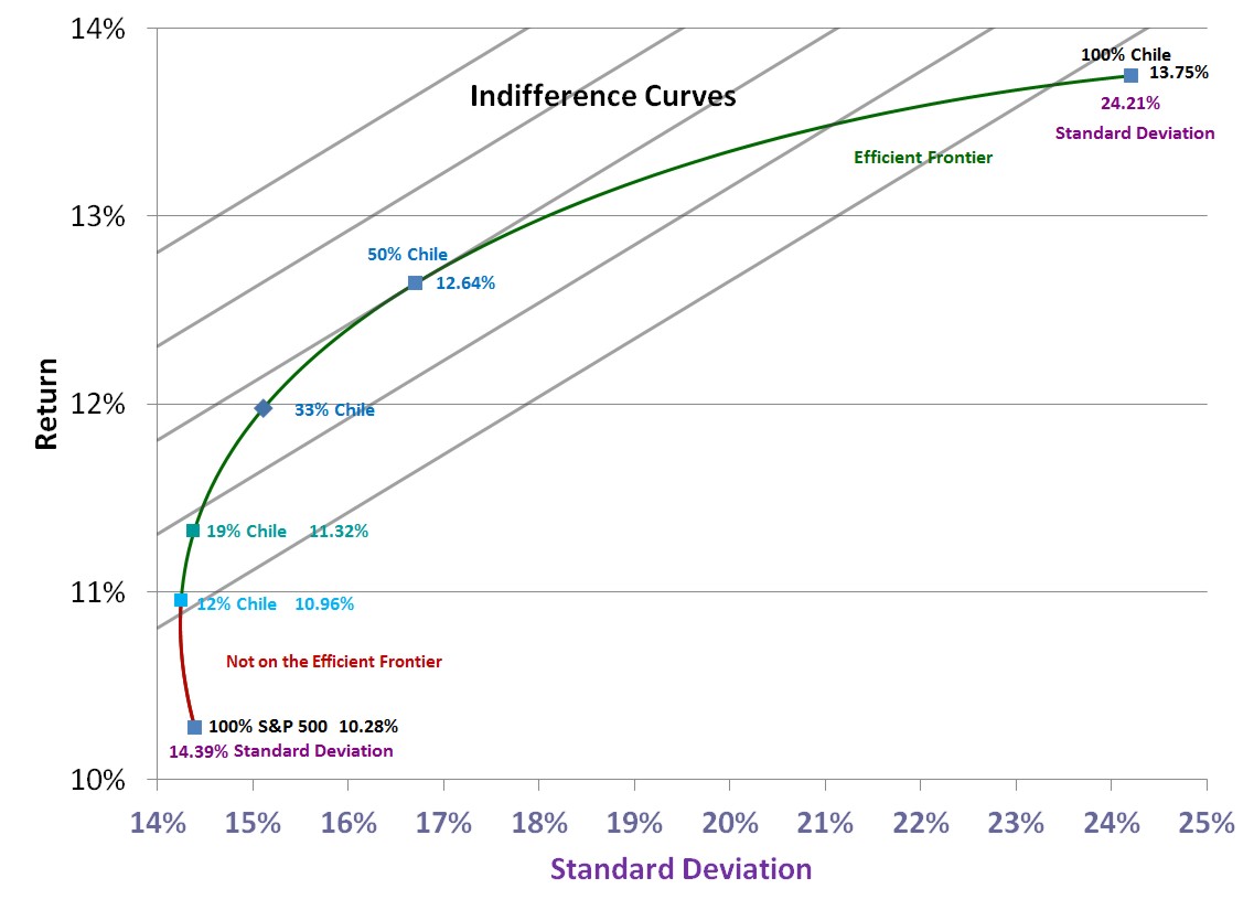
And just to be clear, in reality, most indifference curves are curved as an investor has both less tolerance and less benefit for risk the higher the standard deviation of that risk.

Many investors are not familiar with the idea of Indifference curves because the idea of Indifference curves are not that useful. It is a theoretical concept based on risk tolerance, but savvy advisors instead compute which place on the efficient frontier offers the best chance for a client to meet their goals.

Uses of the Sharpe Ratio are fraught with problems. Here are four basic ones:

1. It isn’t appropriate to use the Sharpe Ratio to choose between two different investment options. It is possible that an investment option may have a lower Sharpe Ration and still be part of a portfolio on the efficient frontier.
2. It isn’t appropriate to use the Sharpe Ratio to choose between different portfolios which are all on the efficient frontier.
3. At best, the Sharpe Ratio is a single hard coded straight-line preference curve, and the portfolio with the highest Sharpe Ratio is not necessarily the one which will give you the best chance of meeting your goals.
4. The Sharpe Ratio arbitrarily uses 1-year standard deviation. For long term investors, one year is a short term measure of volatility that may be inappropriate.